Lab Four: Mini-Final Project

Goals: 
The goal of this lab was to propose a spatial question and to answer that question using Geo-spatial skills learned throughout the semester.  Using four or more Geo-spatial tools created an analysis that was used to make a cartographic map in Arc Map 10.4.1

Introduction:
My proposed spatial question was where would be the best spot to place a new hospital in Eaton County, Michigan? Objectives for this project are that the new hospital should be located within 20 miles of another hospital, within 1 mile of a highway, and near an urban center.  The intended audience would be Eaton County government representatives, as well as local medical facilities and citizens of Eaton County. This question was proposed because I grew up in Eaton County, Michigan and the closest hospital to most of the cities in Eaton County, Michigan is located about 20 miles away making it difficult for people to obtain immediate medical care.

Data Sources:
Data was obtain through the University of Wisconsin-Eau Claire GIS database. Data used was Major highways, Hospitals, Cities, and County feature classes. There were a few data concerns such as if its to big. Another concern was if the data was out of date.

Methods:
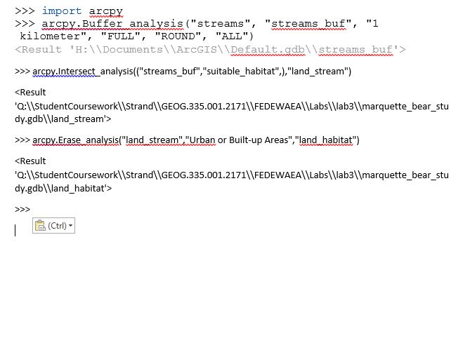
The first thing I did was to add the U.S. states layer from the University of Wisconsin-Eau Claire GIS database. After that, the next step was to create a layer using select by attribute for Michigan.  The next step was to add the highway,cities, county and hospital classes to the map.  The step after that was using the attribute table to only have the highways, as well as cities, and county layers show Michigan.  I created new layers labeled Michigan Hospital, Michigan, Michigan Cities, and Michigan roads. Next I used the Intersect tool on Michigan Hospital and Michigan layers. Using the intersect tool allowed me to combine Michigan Hospital layers with Michigan layers. The following step was using the Buffer tool for all areas around hospital so that new hospitals are away from current ones. This tool allowed me to select a certain distance from the actual location.  The next tool used was the Dissolve tool. This tool was used on the Michigan Hospital buffer, The following tool used was creating a buffer that was within 2 miles of all Michigan cities and in an urban center. I then used the Erase tool on the michigancitybuffer from the hospital buffer. The last tool used was the Dissolve tool on the Michigan hospital buffer.  After the map was created using Arc Map 10.4.1, the next step was to make a data flow model to show the steps mentioned above.

Figure 1: Data Flow Model

Results:

After answering the spatial question using the tools learned in GIS class, it is apparent that the best location for a new hospital in Eaton County, Michigan would be Charlotte City.  Looking at the map posted below, the grey circles represent urban areas that are within 20 miles of a hospital. This location would be near a highway and an urban area. Another location is Grand Ledge, Michigan as well as Mulliken, Michigan.

Figure 2: map results

Evaluation:

My overall impression of this project is that it was good practice to utilize all the current skills learned throughout the course. If asked to do the project again, I would change very little. Although the hardest thing was coming up with a spatial question that wasn't to hard to accomplish with the time given.  Challenges I faced were actually coming up with the spatial question, and figuring what tools to use.

References:
 Data retrieved from "UWEC geospatial data server”.2016.
"Esri - GIS Mapping Software, Solutions, Services, Map Apps, and Data.2016"

    

Lab 3: Vector Analysis

Goals and Background:

There were several goals of this lab. Those goals were to learn how use the geoprocessing tools in Arc Map 10.4.1 for vector data analysis using the Marquette, Michigan geodatabase to determine a suitable habitat for bears. Another goal was using the python scripting in order to farther learn about geoprocessing tools. The last goal of the lab was creating a data flow model to see what geoprocessing tools were used in order to finish the final map project.

Methods:

The first step of this lab was downloading a zip file that contained the geodatabase for Marquette bear study. The next step was to add the X Y coordinate from the bear_locations_geog$ sheet as an event theme. After adding the X Y coordinates to the map, the next step was adding the feature classes within the bear-management_area data-set to the data frame using Arc Map 10.4.1. The following step was to perform a spatial operation that would generate a new feature class to have the ID number of bear and the land cover type. That spatial operation was using the intersect tool. After using the intersect tool to create a new feature class named bear_cover. The next step was to use another spatial tool to find out how many bears were found in each habitat type. In order to find out how many bears were found in each habitat the next spatial tool used was Select By Location using the Minor Type field. Following the Select By Location tool, the next tool was using the Summarize tool in the attribute table. This determines how many bears were located within each habitat section. After performing the previous mentioned tools, it was determined that the bears were located within 3 different habitats. Those three habitats were forest wetlands, evergreen forest land and mixed.

The second step of the lab was to use a spatial tool called Buffer to determine how many bears were located within 500 meters of a stream.  After using the Buffer tool,the next tool used was the Dissolve tool. The following step was using the Intersect tool with  streams and bear cover.  This tool helped determine how many bears were located within 500 meters of a stream.  It was determined that a majority of bears lived within 500 meters of a stream.

The third step of the lab was to find suitable areas for bear habitat based on two criteria. Those criteria s were that it was within a suitable land cover type (one of the 3 habitat mentioned above), and within 500 meters of a stream. The first step in this objective was to create a new feature class using a spatial tool. The spatial operation used was the Intersect tool. By using the Intersect tool with streams, the next step was a dissolve.

The next objective was to exclude all areas that were within 5 kilometers from Urban or Built Up Lands because the Michigan DNR decided that bear management areas should not be in Urban areas. The spatial operations used in this section were the Clip and Erase tools.

After completing the above objectives, the next step was creating the map below to show where a suitable bear habitat might be.

The next objective was to learn how to use python scripting as another geoprocessing method.

The last objective was creating a data flow model to show what geoprocessing tools were used during the making of the map.

Results:
 After completing this lab, it was determined that bears prefer three different types of environments in Marquette County, and that they tend to live closer to streams. The bears also do not live near the Urban areas such as Marquette.

Figure 1: Map of Suitable Bear Habitat using Arc Map 10.4.1

Figure 2: Data Flow Model

    

Figure 3: Python Scripting

References Cited

2016. http://www.dnr.state.mi.us/spatialdatalibrary/metadata/wildlife_mgmt_uni ts.htm.

"Michigan Geographic Framework: Marquette County". 2016. Mcgi.State.Mi.Us. http://www.mcgi.state.mi.us/mgdl/framework/metadata/Marquette.html.

"Michigan 1992 NLCD Shapefile By County". 2016. 

Mcgi.State.Mi.Us. http://www.mcgi.state.mi.us/mgdl/nlcd/metadata/nlcdshp.html.

Lab 2: Downloading GIS Data

Goal:   

The goal of this lab was to learn how to obtain data through online sources, and adding that data using Arc Map 10.4.1 in order to create two different maps. Another goal of this lab was building a web map and share it online. 

Methods: 

The first step to lab two was to visit the census data website and locate the 2010 population data from http://factfinder2.census.gov/faces/nav/jsf/pages/index.xhtml.   After finding 2010 population data from the website, the next step was changing the excel files so that the data would work in Arc Map 10.4.1, in other-words, saving the data as an excel workbook. After saving the excel files as a work book and fixing a few other items, the next step was  downloading shape-files using the website posted above.  After downloading the shape-files, the next step was adding the shape-files and excel workbook to a blank map using Arc Map 10.4.1.  After adding the shape-files and workbook data to the map, the next step was to join data files through Geo#id.  The final step click on properties and change the symbology to graduated colors so that it would be easier to see the represented counties for total population of 2010.

Following the steps mentioned above, is how the second map was created. 

After making the two maps, the next step was to learn how to make a web map.  In order to do that the first step was deleting the second map of housing units and saving the file as a different name. The next step was signing into ArcGIS online through Arc Map 10.4.1. After that, the next step was to sign in onto ArcGIS webpage.  Using the University of Wisconsin- Eau Claire Geography and Anthropology account, the next step was to configure the map. The final step was  publishing the map online. 

Results: 

According to the population map the highest population is in the larger cities. The same goes for the vacant houses. There are more vacant houses in larger cities. 

References: 

(DADS), Data. "American Factfinder". Factfinder2.census.gov. N.p., 2016. Web. 23 Nov. 2016.

(DADS), Data. "American Factfinder". Factfinder2.census.gov. N.p., 2016. Web. 23 Nov. 2016.


    

Extra credit: Geography Week!

  November 14, 2016 was the start of Geography Week, held every fall at the University of Wisconsin- Eau Claire. Throughout the week there are many events including a resume workshop, internship panel, Geography Bee, GIS Day, and several talks held by Alumni.  I was fortunate enough to be able to make it to both GIS day and a talk held by an Alumni by the name of Tunga Chuluunbaatar. 

   GIS day is an event held for several hours where students have the opportunity to give presentations on work that has some kind of geospatial aspect to it, They are doing in various geography classes or research.  I listened to several individuals explain what they are doing in classes such as Quantitative Methods, and Geography Field Seminar.  I also listened to Alex Kleinschmdt talk about his research with Professor Harry Jol over the summer in Lithuania.  Through the use of Ground Penetrating Radar, the team was able to locate a tunnel the Jews used to escape a concentration camp.  My soils class also had someone talking about the work we are doing using LIDAR and GIS as well as other equipment.   I also did research over the summer with Professor Gary Running helping archeologists from the University of Minnesota-Moorhead locate where there could be native American artifacts.  We also used LIDAR and GIS as well as other techniques.  Overall, the event was a great way to showcase what other geography classes are doing as well as various research opportunities that are available for student research! I thought GIS day was a great learning opportunity, and it was neat to see what other students like myself are doing.

   Another event I attended was a talk presented by Tunga Chulunnbaartar.  She graduated from the University of Eau Claire and shared with us her work in Mongolia. In her presentation she shared how they are making multiple maps in a community that is largely cut off from essential needs such as water.  Through communicating with the residents and public officials Tunga and her team were able to make maps and show the community what is needed. For example, they noticed that many students were getting into accidents and hit by vehicles.  Tunga explained to us how her team went into that area, and through talking with the community, public officials, schools, etc. they were able to come up with a solution of how to reduce the number of accidents.  It was a simple solution of having the students go out the back door instead of the front.  They were also able to locate where water access was the most needed.  Another thing Tunga talked about was the amount of garbage built up over time because people didn’t know when the trash would be picked up.  The garbage companies never came through the day.  By showing people maps, and organizing times where garbage would be picked up, they were able to reduce waste!  Overall, Tunga is doing some amazing things with GIS, and communication.  I guess I didn’t realize just how much GIS is used everywhere.  I think geography week is a good event to make people more aware that geography is used more than people think!

Lab 1: Base Data

Lab 1: Base Data

Goals:
The City of Eau Claire, Wisconsin is well known for its concerts and musical festivals throughout the United States. Finding space for those concerts, festivals, and theater productions have become challenging, leaving Eau Claire to search for other options.  The Confluence Projects goal is to provide a multi-million dollar building featuring classrooms, galleries, offices, art studios, and theater production auditoriums. ( http://www.eccommunityfoundation.org/wp-content/uploads/2014/09/Confluence-Brochure-2015-final.pdf)  The goal of this lab was to prepare several base maps that show the location of the confluence project, and to become familiar with different spatial data sets used by public land management, administration, and land use.

Methods:

The first step of this lab was using arc map to digitize the confluence project.  The next step was making six different maps using spatial data from the City of Eau Claire geodatabase, showing the location of the confluence project.  The maps were Civil Divisions, Census Boundaries, Eau Claire City Parcel Data, Zoning, and Voting Districts.

The first map, Civil Divisions, shows different Civil Divisions of Eau Claire County.  The first step to making this map was adding data the base map and choosing the imagery map.  After adding the base map, the next step is to add the county boundary, and civil divisions using the 2009-07-13_EauClaire geodatabase to the base map.  Adjusting the symbology of the civil division shows various municipality types, as well as making the county boundary hollow.  The final step was adding a legend, scale bar, title, and north arrow to help make the map visually appealing.

The second map, Census Boundaries, shows population density of Eau Claire near the proposed site.  The first step to this map was adding the base map and choosing imagery.  The next step was adding the block groups and tracks to the map using 2009-07-13_EauClaire geodatabase and choosing the Census_Features.  In order for the base map to show, making both the block group and track layers transparent is the next step as well as making the tracts layer hollow.  Another step to finalizing the second map was adjusting the symbology of the block groups.  As in the first map, adding a legend, scale bar, title, and north arrow helps make the map visually appealing.

The third map, PLSS Features, uses the Public Land Survey System to show where the proposed site falls within the quarter-quarter sections. The first step to make this map was to add the base map using imagery. The next step was adding the quarter-quarter section using the City of Eau Claire geodatabase.  After adding the quarter-quarter section, the next step was making the quarter-quarter section hollow with a black outline.  The final step was adding a title, legend, north arrow and scale bar.

The fourth map, Eau Claire City Parcel Data, shows the roads in the area around the proposed site as well as parcels.  The first step to add a base map using imagery.  The second step was adding the parcel area, center-lines, and water layers to the base map using the City of Eau Claire geodatabase.  The next step was making the center-line red, and the water green with slightly transparent, and adding the proposed site to the base map layers.  The final step was adding a title, legend, scale bar, and north arrow to the map.

The fifth map, Zoning, shows different businesses surrounding the proposed site.  The first step was the same as the last four maps, adding a base map, using imagery.  The second step was to add the zoning class using the City of Eau Claire geodatabase.  The next step was grouping the different zones together using symbology tab in the properties.  After that, the next step was adding the center-line class to the map. The next step was to change the colors so that it was visually appealing to the reader. The final step was to add the legend, north arrow, scale bar, and title to the map.
The six map, Voting Districts, was made to show where the voting districts are near the proposed site.  As in the other maps, the first step was to add a base map using imagery.  The next step was to add the voting districts feature class to the map. Next was to make the districts different colors and turning on labels so that the numbers appear.  The final step was to add a scale bar and a title to make the map more visually appealing.

Results:
The lab shows the location of the confluence project and the six maps show different feature classes.  The Eau Claire City Parcel Data shows the roads, water around the proposed site.  The Census Boundaries shows the population in the area.  The PLSS data shows different public land used around the area. The zoning map shows different businesses, and residential areas around the proposed site.  The civil divisions map shows the population around the area.  The maps show that the confluence project is a good location and should help bring more business to the City of Eau Claire.